Lecture 01 - Course Introduction, Introduction to PGMs
Course Introductory Admin-related details and an introduction to PGMs in the scope of this course
Logistics
- Class webpage: lengerichlab.github.io/pgm-spring-2025
- Textbooks:
- Daphne Koller and Nir Friedman, Probabilistic Graphical Models
- M. I. Jordan, An Introduction to Probabilistic Graphical Models
- Class Announcements, Assignment Submissions: Canvas
- Instructor: Ben Lengerich
- Office Hours: Thursday 3:30-4:30pm, 7278 Medical Sciences Center
- Email: lengerich@wisc.edu
- TA: Chenyang Jiang
- Office Hours: Monday 11am-12pm, 1219 Medical Sciences Center
- Email: cjiang77@wisc.edu
Course Schedule / Calendar
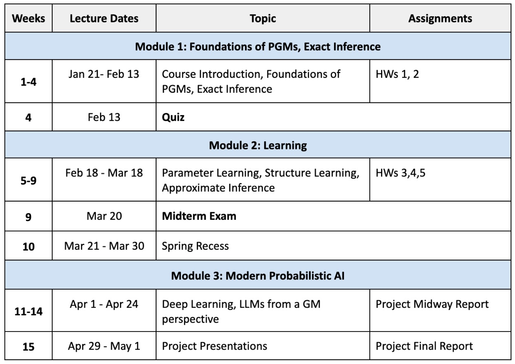
Grading
- HW Assignments (40% of grade)
- Expecting 5 HW Assignments
- All in Modules 1 and 2
- Quiz (40% of grade)
- End of Module 1 (Feb 13)
- Format: In-class, Closed-book.
- Midterm Exam (20% of grade)
- End of Module 2 (Mar 20)
- Format: In-class, Closed-book.
- Final Project (30% of grade)
- Milestones will be due along the way semester
- Lecture Notes (up to 3% extra credit)
Grading Scale
- No curving:
- A: 93–100%
- AB: 88–92%
- B: 83–87%
- BC: 78–82%
- C: 70–77%
- D: 60–69%
- F: Below 60%
Homework Policies
- Expecting 5 HW Assignments
- All in Modules 1 and 2
- Assignments must be submitted via Canvas by the deadline (typically Fridays at 11:59 PM).
- Late submissions will incur a penalty of 10% per day, up to three days, at which they will not be accepted.
- Collaboration: Students may collaborate on understanding the problems, but all submitted work must be individual. Use of AI tools is allowed, but answers must reflect your own understanding. You are responsible for ensuring no plagiarism.
Project
- Proposal (5%): Due Feb 21, 2025. Must outline the group members, problem statement, motivation, dataset(s).
- Midway Report (5%): Due Apr 11, 2025. Build on the proposal to have some preliminary dataset exploration and revised methods.
- Presentation (5%): During the last week of class, students will present their findings in a concise and engaging format.
- Report (15%): Due May 5, 2025. The report should detail the problem, methods, results, and conclusions.
- Collaboration: Teams of up to three students are allowed. Contributions of each individual must be clearly delineated in the report.
Extra Credit: Lecture Notes
- Opportunity: Students can sign up to write lecture notes for each class session. If the notes meet quality standards, students will receive up to 3% extra credit added to their final grade.
- Sign-up sheet
- You are expected to work together with the other scribe to generate 1 note document for the lecture.
- Accepted notes will be hosted on our course webpage (optionally with your name attached, your choice).
- Submission: Lecture notes must be submitted within one week of the session.
- Submit on the GitHub for the course webpage.
- Template is available on the webpage.
Attendance / Participation
- Attendance and participation are expected, though they are not part of the formal grade calculation.
- Contact the instructor in advance of extended absences.
Academic Integrity
- By virtue of enrollment, each student agrees to uphold the high academic standards of the University of Wisconsin–Madison; academic misconduct is behavior that negatively impacts the integrity of the institution. Cheating, fabrication, plagiarism, unauthorized collaboration and helping others commit these previously listed acts are examples of misconduct which may result in disciplinary action. Examples of disciplinary sanctions include, but are not limited to, failure on the assignment/course, written reprimand, disciplinary probation, suspension or expulsion.
Mental Health & Wellbeing
- Students often experience stressors that can impact both their academic experience and personal well-being. These may include mental health concerns, substance misuse, sexual or relationship violence, family circumstances, campus climate, financial matters, among others.
- UW–Madison students are encouraged to learn about and utilize the university’s mental health services and/or other resources as needed. Students can visit uhs.wisc.edu or call University Health Services at (608) 265-5600 to learn more.
Introduction to Probabilistic Graphical Models (PGMs)
What is a Graphical Model?
A graphical model is a technique for representing a probability distribution to make inferences in situations involving uncertainty, which is essential for tasks like speech recognition and computer vision. Typically, we have a dataset consisting of samples: $D = {X_{1}^{(i)},X_{2}^{(i)},…,X_{m}^{(i)} }_{i=1}^N$. The relationships between the elements in each $X$ can be represented by a graph $G$. From this, we derive the model $M_G$.

Graphical models allow us to consider fundamental questions with respect to three branching categories:
- Representation
- How to encode our domain knowledge/assumptions/constraints?
- How to capture/model uncertainties in possible worlds?
- Inference
- How do I answer questions/queries according to my model and/or based on
observed data?
- e.g: $P(X_{i} \mid D)$
- How do I answer questions/queries according to my model and/or based on
observed data?
- Learning
- What model is “right” for my data?
- e.g: $ M = \arg\max_{M \in \mathcal{H}} F(D; M) $
- What model is “right” for my data?
The following section investigates how PGMs help us answer these questions.
Representation:
Joint Probability Distribution of Multiple Variables
The joint probability distribution of a set of random variables represents the probability of all possible combinations of values that the variables can take. Given a set of variables ( X_1, X_2, \dots, X_n ), their joint probability distribution is expressed as:
$ P(X_1, X_2, \dots, X_n) $
This represents the probability that all variables take specific values simultaneously. If the variables are Boolean (i.e., each ( X_i ) can either be 0 or 1), then the joint probability distribution represents the probability of each possible combination of 0s and 1s across the variables.
Example: Joint Probability for a Set of Boolean Variables
Suppose we have a set of Boolean variables $ (X_1, X_2, \dots, X_n) $. These variables can each take values from the set $ { 0, 1 } $. The joint probability distribution would describe the probability of each combination of these 8 variables.
The total number of configurations in this joint probability distribution is:
$ 2^{8} = 256 $
This means there are 256 different possible states for these 8 Boolean variables. For example, one possible configuration might be:
$ X_1 = 0, X_2 = 1, X_3 = 0, \dots, X_8 = 1 $
The probability for this configuration would be:
$ P(X_1 = 0, X_2 = 1, \dots, X_8 = 1) $
Thus, for $n$ Boolean variables, we would have $2^{n}$ possible configurations in the joint probability distribution.
Can We Disallow Certain State Configurations?
Yes, certain state configurations can be disallowed based on domain knowledge, assumptions, or constraints. This can be done either by conditioning the distribution on certain variables or by modifying the joint distribution to set certain configurations to zero probability.
Example: Conditioning and Disallowing Certain Configurations
If we have the same 8 Boolean variables $ X_1, X_2, … , X_8 $, and we know that certain combinations are impossible based on domain constraints, we can condition the joint probability distribution to exclude these configurations.
For example, suppose the configuration $ X_1 = 0, X_2 = 1, X_3 = 0, \dots, X_8 = 1 $ is not possible. We can set:
$ P(X_1 = 0, X_2 = 1, X_3 = 0,…, X_8 = 1) = 0 $
Alternatively, we may choose to focus only on a subset of possible configurations. For example, if we know that $ X_5 $ and $ X_7 $ cannot both be 1 simultaneously, we can redefine the joint distribution as:
This limits the set of allowed configurations to those that respect this constraint.
Focus on Subset of Configurations
It is possible to focus on a subset of configurations by restricting the model. This can be achieved by conditioning the joint probability distribution on a set of variables or by focusing only on valid state configurations.
Example: Conditioning and Subset Focus
If we are only interested in configurations where $ X_1 = 1 $, we can condition the distribution on $ X_1 = 1 $. The resulting probability distribution is then:
This effectively narrows the focus of the distribution to only the cases where $ X_1 = 1 $, and ignores all other configurations of $ X_1 $.
In Markov Models or Markov Decision Processes (MDPs), the model’s assumptions can be used to simplify the dependency structure and focus on specific subsets of states or variables. For example, in MDPs, the agent’s actions may only influence the next state and immediate reward, and the probability distribution over future states may depend only on the current state and action, not the entire history.
By restricting the joint probability distribution, you can focus on the most relevant or feasible configurations in the problem.
Inference
To answer queries like $ P(X_i \mid D) $, we apply Bayes’ Rule:
$ P(X_i \mid D) = \frac{P(X_i, D)}{P(D)} $
Where $ P(X_i, D) $ is the joint probability of $ X_i $ and the observed data $ D $. This is computed by marginalizing over all unobserved variables:
$ P(X_i \mid D) = \frac{\sum_{X_1, \dots, X_n} P(X_1, \dots, X_n, D)}{P(D)} $
Here, the sum is over all possible configurations of the unobserved variables. The denominator $ P(D) $ is the marginal likelihood.
In simpler cases, if the variables are independent, the joint distribution factorizes. For instance, if $ X_i $ is independent of other variables, then:
$ P(X_i \mid D) = P(X_i) $
This reduces the computation, as we don’t need to sum over other variables.
Graphical models like Bayesian Networks exploit conditional independencies between variables, allowing us to factorize the joint distribution:
$ P(X_1, \dots, X_n) = \prod_{i} P(X_i \mid \text{parents}(X_i)) $
This structure simplifies inference by reducing the number of configurations to sum over, making it more efficient.
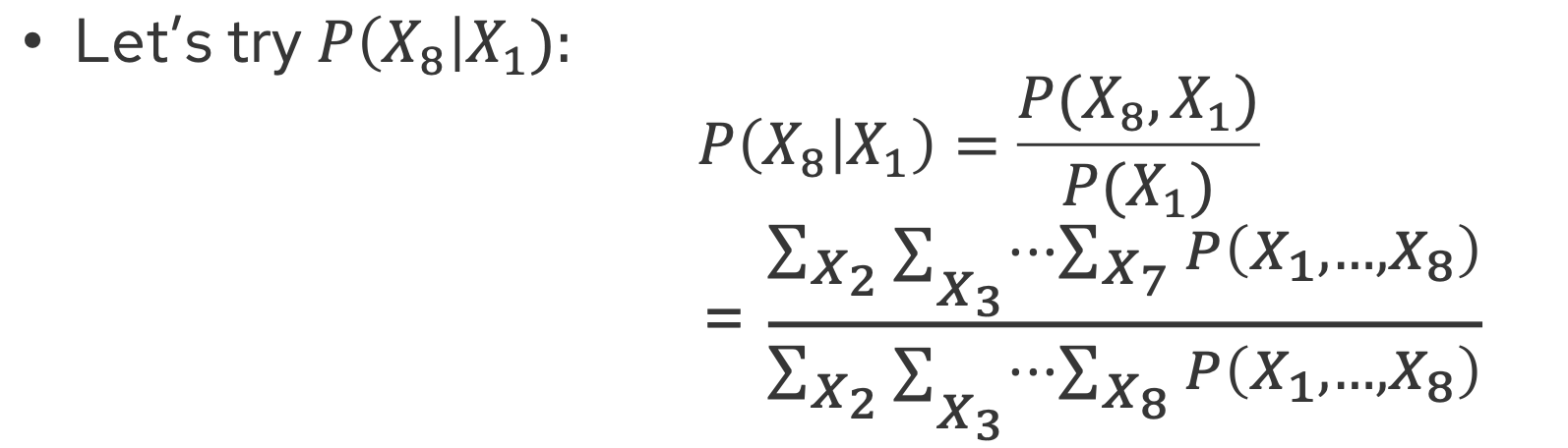
Note: If all $ X_i are independent, P(X_8 \mid X_1) = P(X_8) $.
As a more specific case, view the sample calculation below:
Learning: Finding the Right Model
When we talk about learning in the context of probabilistic models, we usually aim to choose the model $ M $ from a set of possible models $ \mathcal{H} $ that best explains or fits the observed data $ D $.
The goal is to find the model $ M $ that maximizes some objective function, typically the likelihood of the data, or some score function, denoted as $ F(D; M) $. This can be written as:
$ M = \arg\max_{M \in \mathcal{H}} F(D; M) $
Where:
- $ M $ is the model we are selecting.
- $ \mathcal{H} $ is the hypothesis space, which is the set of all possible models.
- $ F(D; M) $ is a function that evaluates how well model $ M $ explains the data $ D $ (e.g., likelihood, Bayesian posterior, or another scoring function).
- $ \arg\max $ means we are finding the model $ M $ that maximizes $ F(D; M) $.
Constraining the Hypothesis Space $ \mathcal{H} $
To make the search for the optimal model more efficient, we need to constrain the hypothesis space $ \mathcal{H} $. Without constraints, the space of possible models may be too large to search efficiently.
Suggested methods to Constrain $ \mathcal{H} $:
-
Prior Knowledge: Use domain knowledge to narrow down the set of possible models. This could involve specifying certain structures, such as limiting the models to certain types of graphical models (e.g., Bayesian networks, Markov chains) or making assumptions about the data (e.g., assuming Gaussian distributions).
- Regularization: Apply regularization techniques to prevent overfitting and guide the search for simpler models. This can include:
- L1 regularization (Lasso) or L2 regularization (Ridge) to penalize large model parameters.
- Bayesian priors that favor certain kinds of models over others.
-
Model Family: Instead of searching over all possible models, restrict the search to a family of models (e.g., linear regression, decision trees, etc.), which reduces the hypothesis space $ \mathcal{H} $.
- Simplifying Assumptions: For instance, in graphical models, you might assume conditional independence between certain variables to reduce the complexity of the search space.
Example of how imposing a dependency structure simplifies representation of a PGM of the inside of a cell:
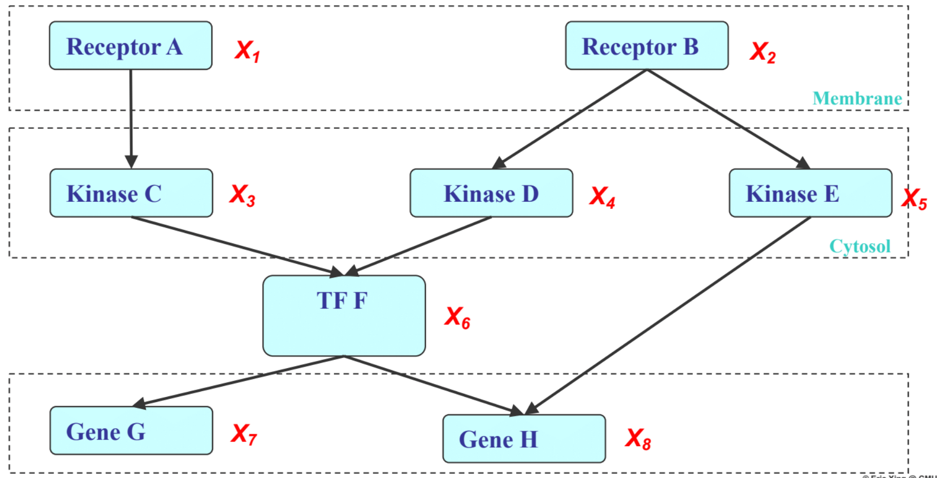
- If the $X$’s are conditional independence (as encoded by a PGM), then the joint can be factorized into a product of simpler terms:
The benefits of this representation are listed below.
Why PGMs?
-
Incorporation of domain knowledge and causal (logical) structures
PGMs allow you to directly encode domain knowledge and causal relationships into the model. This makes it easier to represent real-world dependencies, such as how diseases cause symptoms or how different factors influence one another. -
Learning domain knowledge and causal structures from data
PGMs can learn new relationships from data, automatically detecting dependencies, correlations, and causal links, which makes them adaptable to new, unseen data or changing environments. -
Modular combination of heterogeneous parts – data fusion
PGMs can combine data from multiple sources (e.g., sensors, behaviors, environmental factors) into a unified model, allowing for data fusion that improves accuracy and provides a comprehensive view of the system. -
Bayesian Learning – can easily incorporate uncertainty, and can be specific to a particular part of the model
PGMs use Bayesian learning to incorporate uncertainty into the model, representing probabilities rather than hard predictions. This allows for localized uncertainty in specific variables or components without affecting the whole model.
How does a PGM differ from a GM?
- PGM = Multivariate Statistics + Structure
-
GM = Multivariate Objective Function + Structure
- Formally: A PGM is a family of distributions on a set of random variables that are compatible with all the probabilistic independence propositions encoded by a graph that connects these variables.
The two types of GMs are:
- Directed edges give causality relationships (Bayesian Network or Directed Graphical Model)
- Undirected edges simply give correlations between variables (Markov Random Field or Undirected Graphical model):
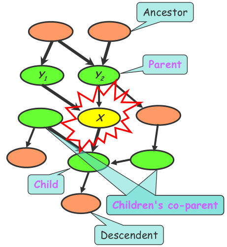
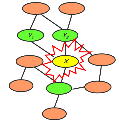
For instance, the Bayes net uses a directed acyclic graph (DAG). Each node in a Bayes net has a Markov blanket, composed of its parents, its children, and its children’s parents. Every node is conditionally independent of the nodes outside its Markov Blanket. Therefore, the local conditional probabilities as well as the graph structure completely determine the joint probability distribution. This model represents causality relationships can be used to generate new data.They are acyclic in order to ensure no feedback loops, maintaining a clear causality structure.
By contrast, the Markov random field uses an undirected graph. Every node is conditionally independent of the other graph nodes, except for its immediate neighbors. To determine the joint probability distribution, we need to know local contingency functions as well as structural cliques. This model represents correlation between variables, but cannot explicitly generate new data. Note that these structures can include cycles, unlike Bayesian Networks.
Towards structural specification of probability distributions
- Separation properties in the graph imply independence properties about the associated variables.
- For the graph to be useful, any conditional independence properties we can derive from the graph should hold for the probability distribution that the graph represents.
- The Equivalence Theorem:
- For a graph $ G $,
- Let $ D_1 $ denote the family of all distributions that satisfy $ I(G) $,
- Let $ D_2 $ denote the family of all distributions that factor according to $ G $,
- Then $ D_1 \equiv D_2 $.
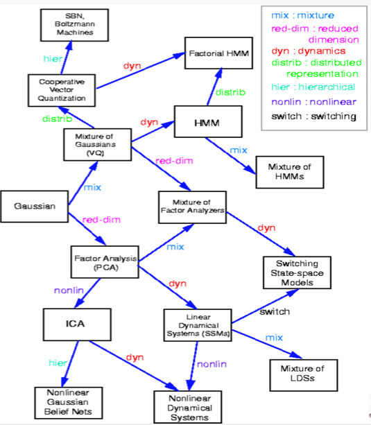
A brief elucidation of the evolution and key developments of graphical models over time may be necessary. View the incomplete genealogy of GMs below:
Fancier GMs
GMs can be applied in numerous more advanced ways to solve complex problems in areas like reinforcement learning, machine translation, etc.
Why GMs?
-
What’s the point of GMs in the AI era?
GMs enable efficient handling of uncertainty and complex dependencies in AI systems, making them essential for decision-making and predictive modeling. -
A language for communication
GMs offer a clear, visual framework to represent probabilistic relationships, facilitating communication across domains and stakeholders. -
A language for computation
GMs provide efficient algorithms for probabilistic inference, enabling scalable and precise predictions in complex systems. -
A language for development
GMs support modular model design, making it easier to build, experiment with, and refine AI systems with probabilistic reasoning.