Lecture 03 - A Linear View of Discriminative and Generative Models
Introduction to LaTex & Distinction between Discriminative and Generative Models
Logistics Review
- Lecture scribe sign-up sheet
- Instructor: Ben Lengerich
- Office Hours: Thursday 2:30-3:30pm, 7278 Medical Sciences Center
- Email: lengerich@wisc.edu
- TA: Chenyang Jiang
- Office Hours: Monday 11am-12pm, 1219 Medical Sciences Center
- Email: cjiang77@wisc.edu
Homework info
- Released: Due Friday at midnight.
- Submit via: Canvas
Introduction to LaTeX
What is LaTeX
- LaTeX is a document preparation system and markup language designed for creating high-quality documents.
- Key Ideas:
- Separation of content and formatting.
- Not WYSIWYG (like Word); instead, uses precise design commands.
- Implications:
- Handles complex layouts like tables, equations, and citations seamlessly.
- Some upfront work, but no fighting the system for layout.
Why Use LaTeX
- Professional Output: Superior typesetting for academic papers, theses, and technical reports.
- Handles Complexities: Simplifies math formulas, bibliographies, and cross-referencing.
- Automation: Automatically generates tables of contents, indices, and citations.
- Reproducibility: Consistent document appearance across different platforms.
Basics of a LaTeX Document
- Preamble: Sets up document type and packages.
\documentclass{article} \usepackage[utf8]{inputenc} - Content: The body of your document.
\begin{document}
Hello, World!
\end{document}
Essential Commands
- Text Formatting:
- Bold:
\textbf{bold text} - Italics:
\textit{italic text} - Underline:
\underline{text}
- Bold:
- Lists:
\begin{itemize}
\item Item 1
\item Item 2
\end{itemize}
Math in LaTeX
- In-line math: Single $ to start/end math environment:
$E = mc^2$ - Block math:
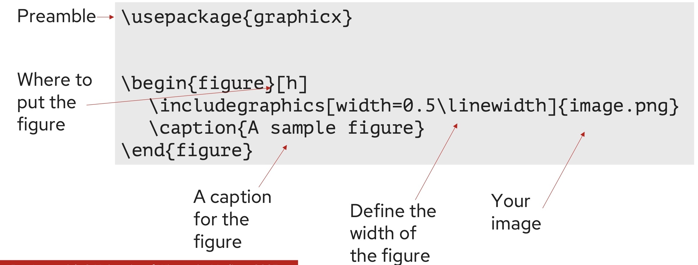
\[
E = mc^2
\]
Figures
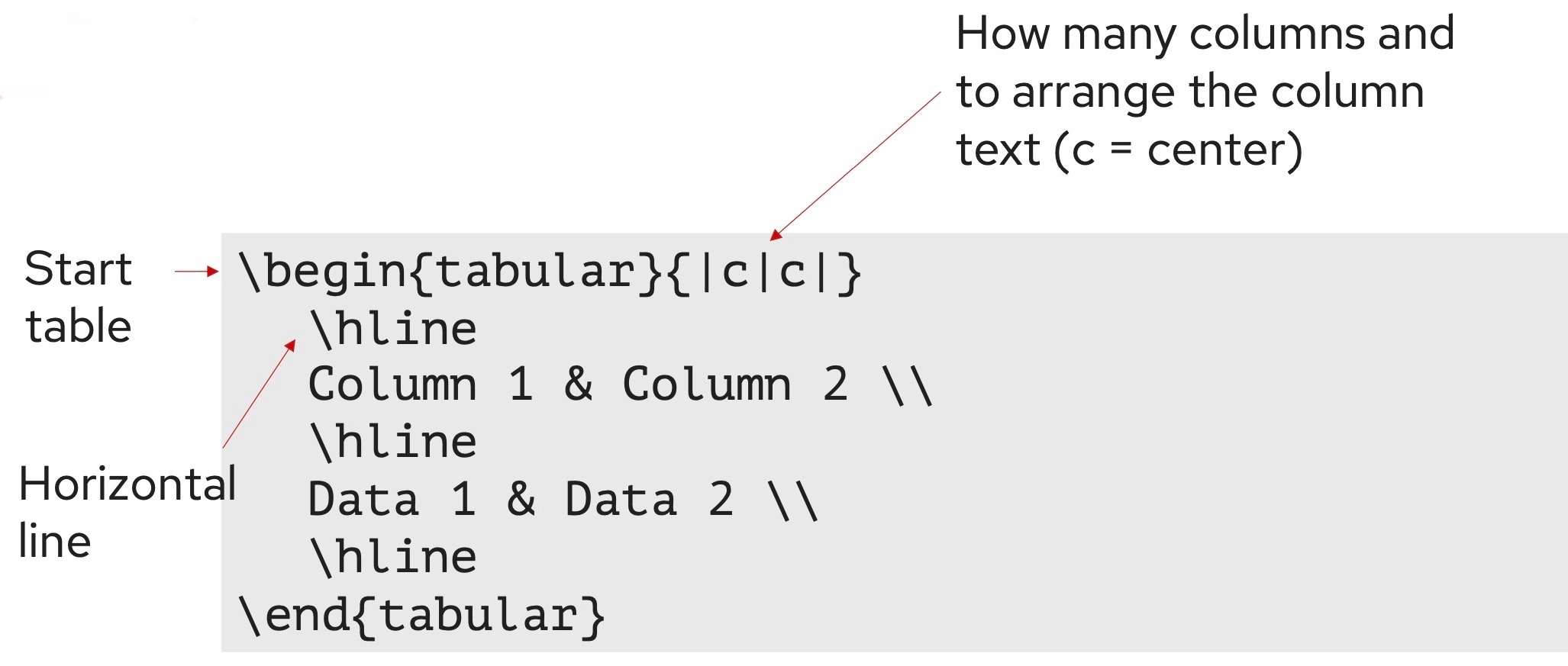
Tables
Where to Use LaTeX
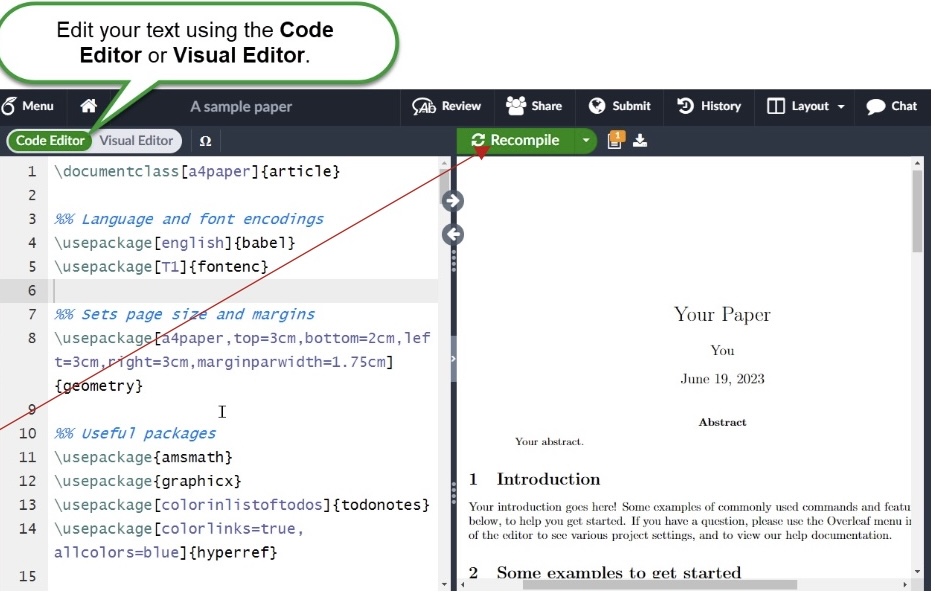
- Overleaf: Recommended for live collaboration and automatic backups.
- Local Editors: TeXShop, MikTeX, TeXworks.
- Workflow:
- Write LaTeX code.
- Compile using the “Recompile” button on Overleaf or with
pdflatex/xelatexlocally. - View and iterate on the generated PDF.
Resources
Discriminative and Generative Models
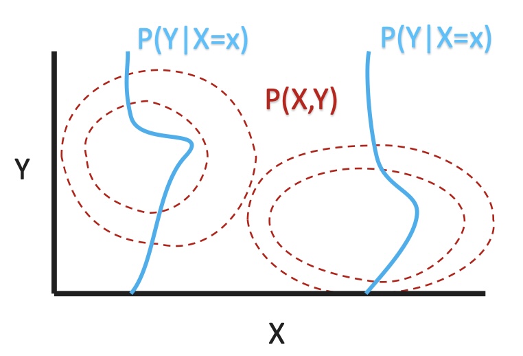
Generative Models: Model the joint distribution, $P(X, Y)$. They aim to model the underlying data distribution Discriminative models: Models the conditional distribution, $P(Y\mid X)$. They focus on just distinguishing between different classes.
The discriminative and Generative Path to $P(Y\mid X)$:
Both Discriminitve and generative models end at $P(Y\mid X)$ but they get there in different ways.
Generative Models Observe X and Y, then learn $P(X\mid Y)$, $P(Y)$ and calculate $P(X) = \int P(X,Y) \, dY$. Then, use these to calcualate $P(Y\mid X) = \frac{P(X\mid Y)P(Y)}{P(X)}$. When looking to calculate $\hat{Y}$, we just need to learn $P(X\mid Y)$ and $P(Y)$. Then we can calculate $\hat{Y} = \arg\max P(X\mid Y) \cdot P(Y)$
Discriminitive Models Observe X and Y, and then learn $P(Y\mid X)$ . It is a more straightforward approach, but you do not learn as much about X, Y and their distributions. Similarily, if we are looking to get $\hat{Y}$ from observing X and Y, we can learn $P(X \mid Y)$ and use it calculate $\hat{Y} = \arg\max P(Y\mid X)$
Example Discriminative Model - Logistic Regression:
Our goal here is to observe X and Y and from them learn $P(Y\mid X)$. We do this through Parameterization:
- $P(Y = 1\mid X) = \sigma(\theta^T X)$, where $\sigma(z) = \frac{1}{1 + e^{-z}}$ is the sigmoid function.
- $P(Y = 0\mid X) = 1 - P(Y = 1\mid X)$
Why do we do this parameterization? If we take the log-odds and simplify, we get: $\log \left( \frac{P(Y = 1 | X)}{P(Y = 0 | X)} \right) = \theta^T X$ .
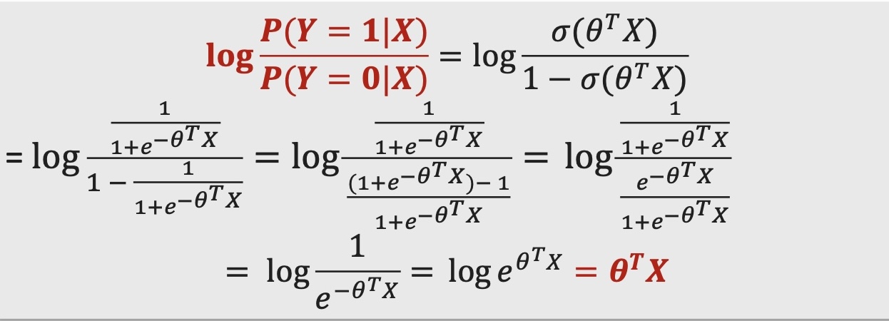
This provides a linear relationship between the input features X and the log-odds of the outcome Y. By using the sigmoid function, we map this linear relationship to the probability space, ensuring that the predicted probability lies between 0 and 1.
Using these paramterizations, we can calculate $\hat{\theta}$ from observations of X and Y in our data: $\hat{\theta} = \arg\max \prod_{i} P(Y_i \mid X_i; \theta) = \arg\max \sum_{i} \left( Y_i \log \sigma(\theta^T X_i) + (1 - Y_i) \log (1 - \sigma(\theta^T X_i)) \right)$
Example Generative Model - Naive Bayes:
Our goal here is to observe X and Y and from there learn $P(X\mid Y)$ & $P(Y)$ and calculate $P(X) = \int P(X, Y) \, dY$. Then, use these to calcualate $P(Y\mid X) = \frac{P(X\mid Y)P(Y)}{P(X)}$. We do this through Parameterization:
- $P(X\mid Y) = \prod_{j=1}^{d} P(X_j\mid Y)$
- $P(Y = k) = \frac{\text{number of samples with Y = k}}{\text{total samples}}$
- $P(X_j\mid Y) = N(\mu_{jk}, \sigma_{jk}^2)$
A note on this parameterization? This is making the assumption of condtional Independence of the features in $X_1, X_2, \dots, X_n$ given the class label Y. This allows it to simplify the join probability as the product of individual feature probabilities, as is shown in the first bullet. This assumption is why it is the “Naive” Bayes.
Using these paramterizations, we can calculate $\hat{\mu}, \hat{\sigma}$ and from observations of X and Y in our data: $\hat{\mu}, \hat{\sigma} = \arg\max_{\mu, \sigma} P(X\mid Y)$ $P(Y = 1\mid X) = \frac{\prod_{j=1}^{d} P(X_j\mid Y=1) P(Y=1)}{P(X)}$
What about MAP/Regularization:
When we observe X and Y and learn $P(Y\mid X; \sigma)$, $P(\theta)$ in MAP. Our Parameterization stays the same:
- $P(Y = 1\mid X) = \sigma(\theta^T X)$, where $\sigma(z) = \frac{1}{1 + e^{-z}}$ is the sigmoid function.
- $P(Y = 0\mid X) = 1 - P(Y = 1\mid X)$
From there, we estimate $\hat{\theta}$ from observations: $\hat{\theta} = \arg \max \prod_{i} P(Y_i\mid X_i; \theta) P(\theta) = \arg \max_i \sum_{i} \left[ Y_i \log \sigma(\theta^T X_i) + (1 - Y_i) \log(1 - \sigma(\theta^T X_i)) \right] - R(\theta)$
Then, we calaculate $P(Y\mid X)$
Discriminitive vs Generative Models:
Disciminative Models optimize the conditional likelihood: $\hat{\theta} = \arg\max_{\theta} P(Y\mid X; \theta) = \arg\max_{\theta} \frac{P(X\mid Y; \theta)P(Y; \theta)}{P(X; \theta)}$ Generative Models optimize the joint likelihood: $\hat{\theta} = \arg\max_{\theta} P(X, Y; \theta) = \arg\max_{\theta} P(X\mid Y; \theta) P(Y; \theta)$
Are these the same optimization? Only when $P(X; \theta)$ is invaraiant to $\theta$, as $\arg\max_{\theta} \frac{P(X | Y; \theta) P(Y; \theta)}{P(X; \theta)} = \arg\max_{\theta} P(X\mid Y; \theta) P(Y; \theta)$
Summary of Logistic Regression vs Naive Bayes:
| Model | Logistic Regression | Naïve Bayes |
|---|---|---|
| Defines | $P(Y\mid X; \theta)$ | $P(X, Y; \theta)$ |
| Estimates | $\hat{\theta} = \arg\max P(Y \mid X; \theta)$ | $\hat{\theta} = \arg\max P(X\mid Y; \theta) P(Y)$ |
| Asymptotic Error | Lower asymptotic error on classification | Higher asymptotic error on classification |
| Convergence Speed | Slower convergence in terms of samples | Faster convergence in terms of samples |
Andrew Ng’s Insights
Discriminative learning generally leads to lower error in the long run, but a generative classifier can reach its higher error rate more quickly as it learns. In other words, while discriminative models may perform better overall, generative models might be able to learn and converge faster, even if they don’t ultimately achieve the same level of accuracy. Why is this?
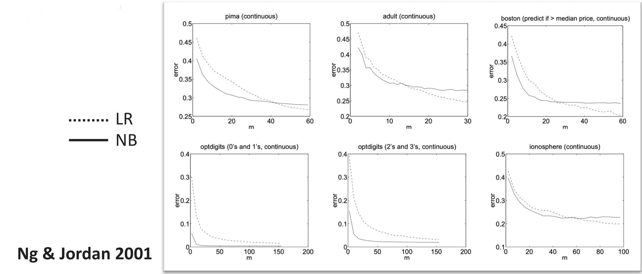
“While discriminative learning has lower asymptotic error, a generative classifier may also approach its (higher) asymptotic error much faster.” The assumptions of this statement:
- Generative models, such as those that estimate $( P(X, Y, \theta) )$, typically make more assumptions to simplify the problem compared to discriminative models that focus on $( P(Y\mid X) )$.
- However, this isn’t always the case.
- Currently, there is no universally correct or general rule for deciding whether to use a discriminative or generative approach to classify an observation $( x )$ into a class $( y )$; the decision depends on how confident we are in the accuracy of the specification of either $( p(y\mid x) )$ or $( p(x, y) )$ for the data.