Lecture 04 - Conditional Independence and Directed GMs (BNs)

Review of conditional independence, and an introduction to Directed GMs (BNs)

• Logistics Review
• Homework info
• Conditional Independence
• Naïve Bayes Classifier
• Bayesian Networks (BNs)
• Hidden Markov Models (HMMs)

Logistics Review

• Class webpage: lengerichlab.github.io/pgm-spring-2025
• Lecture scribe sign-up sheet
• Readings,Class Announcements, Assignment Submissions: Canvas
• Instructor: Ben Lengerich
  • Office Hours: Thursday 3:30-4:30pm, 7278 Medical Sciences Center
  • Email: lengerich@wisc.edu
• TA: Chenyang Jiang
  • Office Hours: Monday 11am-12pm, 1219 Medical Sciences Center
  • Email: cjiang77@wisc.edu

HomeWork info

• Released: Due February 11 at midnight.
  • PDF and Latex solution template (.tex) available on website.
• Submit via: Canvas
• Most preferred format:
  • PDF with your solution written in the provided solution box using LaTeX.

---

Conditional Independence

Definitions

• Independence:
  Variables $X$ and $Y$ are independent $(X \perp Y)$ if:
  • $P(X, Y) = P(X)P(Y)$
• Conditional Independence:
  $X$ and $Y$ are conditionally independent given $Z$ if:
  • $P(X, Y \mid Z) = P(X \mid Z)P(Y \mid Z)$

Example

• Medical Diagnosis:
  Let $X = \text{Fever}, Y = \text{Rash}, Z = \text{Measles}$.
  If a patient has measles ($Z$), knowing they have a fever ($X$) provides no additional information about whether they develop a rash ($Y$).

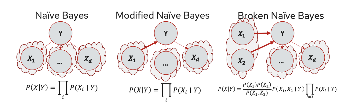
Relate to Naïve Bayes

• Conditional independence allows us to compute $P(X\mid Y)$ efficiently.
• Switching the direction of one arrow does not change the probability.
• Switching the direction of two arrow changes the probability because there is a double-count evidence (two $X$’s repeatedly contains part of information about $Y$)

---

Directed Graphical Models (causality relationship)

Two types of GMs:

• Directed edges give causality relationship (e.g. Bayesian Network)
• Undirected edges give correlations between variables (e.g. Markov Random Field)

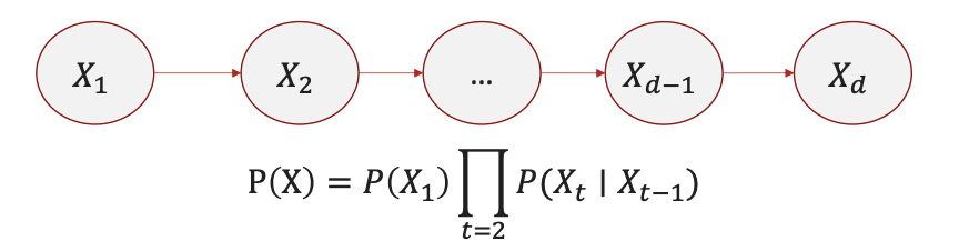
  1. Markov Chains

• Markov Property:
  The future state depends only on the current state:
  • $P(Z_{t+1} \mid Z_t, Z_{t-1}, \ldots) = P(Z_{t+1} \mid Z_t)$
• Transition Matrix:
  Defines probabilities $P(Z_t \mid Z_{t-1})$.
• Application:
  Modeling sequences like weather patterns or stock prices.

2. Hidden Markov Models (HMMs)

We need it when the underlying drivers are not observed

• Components:
  • Hidden States ($Z_t$): Latent variables (e.g., emotional states in speech).
  • Observations ($X_t$): Observed data (e.g., audio signals).
  • Transition Probability: $P(Z_t \mid Z_{t-1})$.
  • Emission Probability: $P(X_t \mid Z_t)$.
• Example:
  Dishonest Casino:
  • Hidden states: Fair die ($Z=0$) vs. loaded die ($Z=1$).
  • Observations: Dice rolls (e.g., $X=6$).
  • Goal: Infer when the dealer switches dice based on observed rolls.

3. Bayesian Networks (BNs)

• Structure:
  A BN is a directed acyclic graph whose nodes represent the random variables and whose edges represent direct influence of one variable on another. Provides the skeleton for representing a joint distribution compactly in a factorized way. It compacts representation of a set of conditional independence assumptions. We can view the graph as encoding a generative sampling process executed by nature.
• Factorization:
  Joint distribution factorizes as:
  • $P(X_1, \ldots, X_n) = \prod_{i=1}^n P(X_i \mid \text{Parents}(X_i))$
• Key Structures:
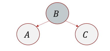
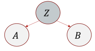
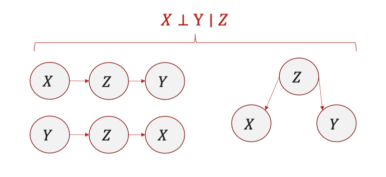
  • Common Parent:
    $A \leftarrow B \rightarrow C$ ⟹ $A \perp C \mid B$.
    Example: $B = \text{Season}, A = \text{Rain}, C = \text{Sprinkler}$.

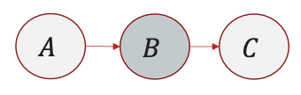
• Cascade:
  $A \rightarrow B \rightarrow C$ ⟹ $A \perp C \mid B$.
  Example: $A = \text{Smoking}, B = \text{Lung Damage}, C = \text{Cough}$.

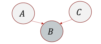
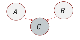
• V-Structure (Collider):
  $A \rightarrow B \leftarrow C$ ⟹ $A$ and $C$ become dependent if $B$ is observed.
  Example: $A = \text{Alarm}, B = \text{Burglary}, C = \text{Earthquake}$.

• I-map
  • Independence set: let $P$ be a distribution on $X$. Define $I(P)$ to be the set of independences $(X \perp Y \mid Z)$ that hold in $P$.
  • I-Map: Let $G$ be any graph object with an associated independence set $I(G)$. We say that $G$ is an I-map for an independent set $I$ if $I(G) \subseteq I$.
  • I-Map Distribution: We say $G$ is an I-map for $P$ if $G$ is an I-map for $I(P)$, when we use $I(G)$ as the associated independence set.

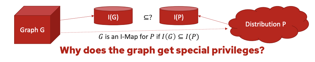
• Facts:
  • Any independence that $G$ asserts must hold in $P$. Conversely, $P$ could contain other independence that are not in $G$.
  • We are capable to use $G$ to estimate $P$.
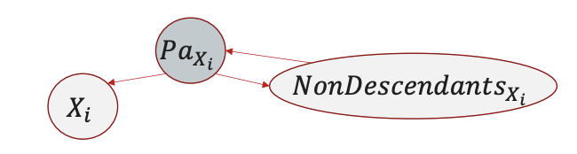
  • Due to the property of BNs, $I(G)$ can be used to represent the local Markov assumption by $I_l(G)={X_i \perp NonDescendants_{X_i} \mid Pa_{X_i}:\forall i}$

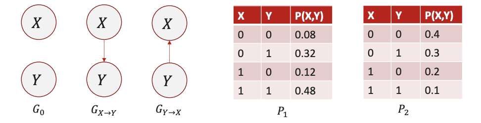
• Example: $G_0$, $G_1$, $G_2$ can be I-map for $P_1$, while $G_0$ is not the I-map for $P_2$. Because $G$ implies independence that is not contained in $P_2$, so it cannot be used to estimate $P_2$.

• D-Separation:
  • A path between $X$ and $Y$ is blocked by $Z$ if:
    1. Chain $\rightarrow \bullet \rightarrow$: Middle node is in $Z$.
    2. Fork $\leftarrow \bullet \rightarrow$: Middle node is in $Z$.
    3. Collider $\rightarrow \bullet \leftarrow$: Middle node and its descendants are not in $Z$.

• Definition: $X$ and $Y$ are d-separated given $Z$ if all paths are blocked.
• MAG definition of D-Separation: Variable $X$ and $Y$ are D-separated given $Z$ if they are separated in the moralized ancestral graph.

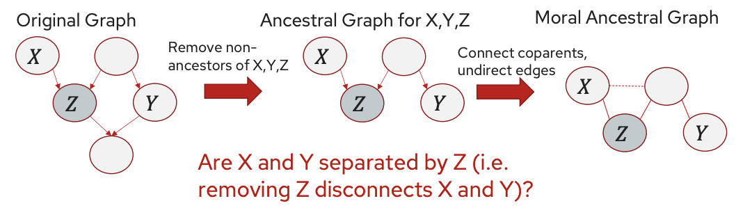
• Example:

---

Learning & Inference

Learning in BNs

• Parameter Learning:
  Estimate Conditional Probability Tables (CPTs) from data:
  • $P(X_i \mid \text{Parents}(X_i)) = \frac{\text{Count}(X_i, \text{Parents}(X_i))}{\text{Count}(\text{Parents}(X_i))}$
• Structure Learning:
  Use algorithms like K2 or PC to infer the DAG from data.

Inference in BNs

• Exact Inference:
  • Variable Elimination: Marginalize variables step-by-step.
  • Junction Tree Algorithm: Transform the BN into a tree structure.
• Approximate Inference:
  • Sampling: Markov Chain Monte Carlo (MCMC).
  • Loopy Belief Propagation: Message-passing in cyclic graphs.

---

I-Equivalence

Definition

• Two Bayesian Networks are I-equivalent if they encode the same set of conditional independence statements.
• Example:
  Networks $A \rightarrow B \rightarrow C$ and $A \leftarrow B \leftarrow C$ are I-equivalent.

Implications

• Different graph structures can represent identical independence relationships.
• Critical for model selection and avoiding overfitting.

Notation: “Plate”

• Naïve Bayes with Streamlined Notation:

---

Applications

1. Naïve Bayes Classifier

• Assumption: Features are conditionally independent given the class.
• Formula:
  • $P(Y \mid X_1, \ldots, X_n) \propto P(Y) \prod_{i=1}^n P(X_i \mid Y)$
• Use Case: Spam detection, sentiment analysis.

2. Hidden Markov Models

• Applications:
  • Speech recognition (mapping audio to words).
  • Bioinformatics (gene prediction from DNA sequences).

3. Causal Inference

• Bayesian Networks for Causality:
  • Identify causal effects using interventions.
  • Example: Estimating the effect of a drug on recovery while controlling for confounders.

---