Lecture 18 - Deep Generative Models

Introduction to Variational Autoencoders, Generative Adversarial Networks, and Diffusion Models.

Logistics Review

• Class webpage: lengerichlab.github.io/pgm-spring-2025
• Instructor: Ben Lengerich
  • Office Hours: Thursday 3:30-4:30pm, 7278 Medical Sciences Center
  • Email: lengerich@wisc.edu
• TA: Chenyang Jiang
  • Office Hours: Monday 11am-12pm, 1219 Medical Sciences Center
  • Email: cjiang77@wisc.edu

Deep Generative Models

Recall Generative and Discriminative models

• Generative:

  1. model joint distribution P(X,Y)
  2. Observe X and Y. Learn P(X|Y) and P(Y).
  3. Calculate P(X) by integrating P(X,Y) over Y, and eventually gets P(Y|X)
  

  • Example: Naive Bayes

• Discriminative:

  1. model conditional distribution P(Y|X)
  2. Observe X and Y and learn P(Y|X)
  

  • Example: logistic regression

What are Deep Generative Models?

• Deep means many layers: $Z_{1}\to …\to Z_{k}\to X$
• Define probablistic distributions over a set of variables.

Early Forms of DGMs:

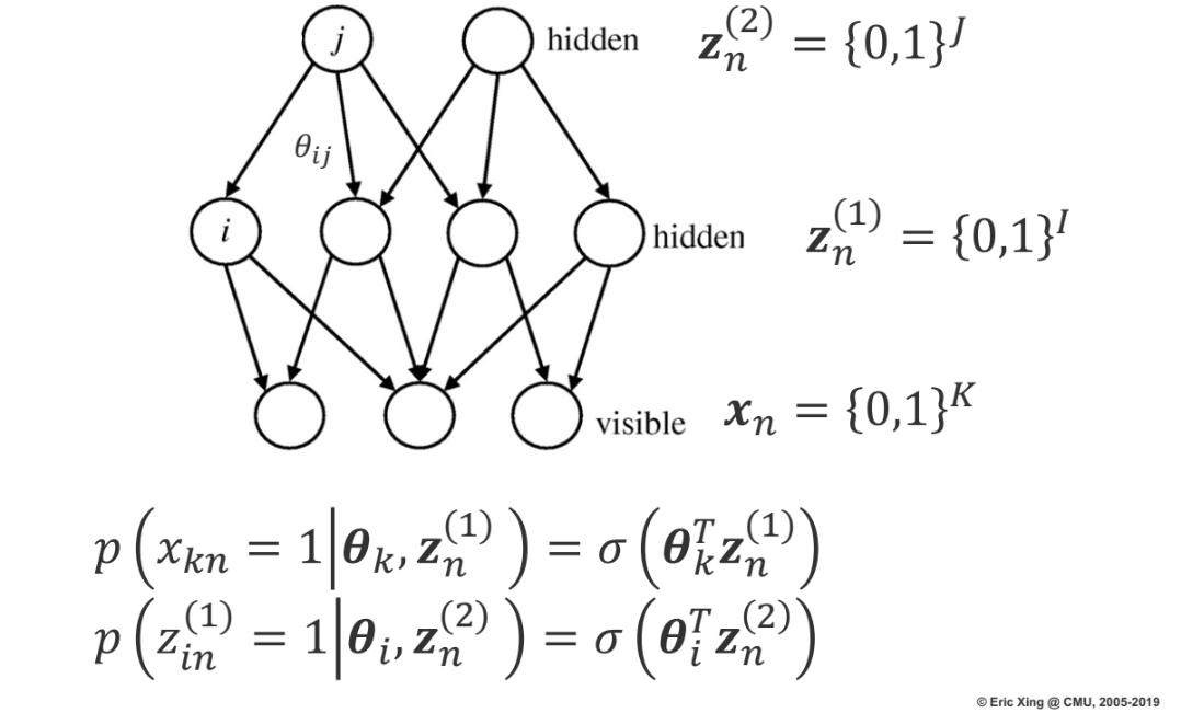
A Probablistic nerual network that uses sigmoid activation functiona to model conditional probabilities. It uses directed edges where nodes are consisted of binary values.

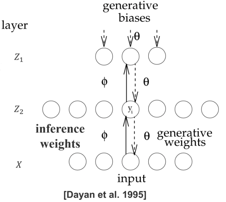
Helmholtz machine has two networks as seen in the graph above. One is bottom-up that takes inputs and produces distributions over hidden layers. Another is top-down that generates values.

How DGMs are trained?

• Via EM framework:
  • E-step (Expectation): Estimate the posterior distribution of the latent variables given the observed data.
  • M-step (Maximization): Maximize the expected log-likelihood with respect to model parameters.
• Sampling and Data Augmentation:
  • Ancestral sampling (for autoregressive models)
  • Gibbs sampling (for undirected models)
• Variational Inference:
  • Replace the true posterior with a simpler distribution.
  • Used in models like Variational Autoencoders.
  • Optimize the Evidence Lower Bound (ELBO):

\[\log p(x) \geq \mathbb{E}_{q(z \mid x)}\left[ \log p(x \mid z) \right] - \mathrm{KL}\left( q(z \mid x) \,\|\, p(z) \right)\]

• Wake and Sleep Algorithm:
  • Wake phase:
    • Use real data to update the generative model.

    • $E_{q(z

      x)}[\log p(x

      z)]$

  • Sleep phase:
    • Use generated data to train the inference model.

    • $E_{q(x

      z)}[\log p(z

      x)]$

Variational Autoencoders (VAEs)

VAEs is variational inference plus autoencoders

Recall ELBO of VI where we let q(z

x) be some family that’s easier to optimize:

\[\log p(x) \geq E_{z \sim q(z)}[\log p(x, z)] + H(q)\]

Also, recall autoencoder:

1. Use encoder to compress data into smaller details.
2. Pass through latent space.
3. Use decoder to recreate the original input.

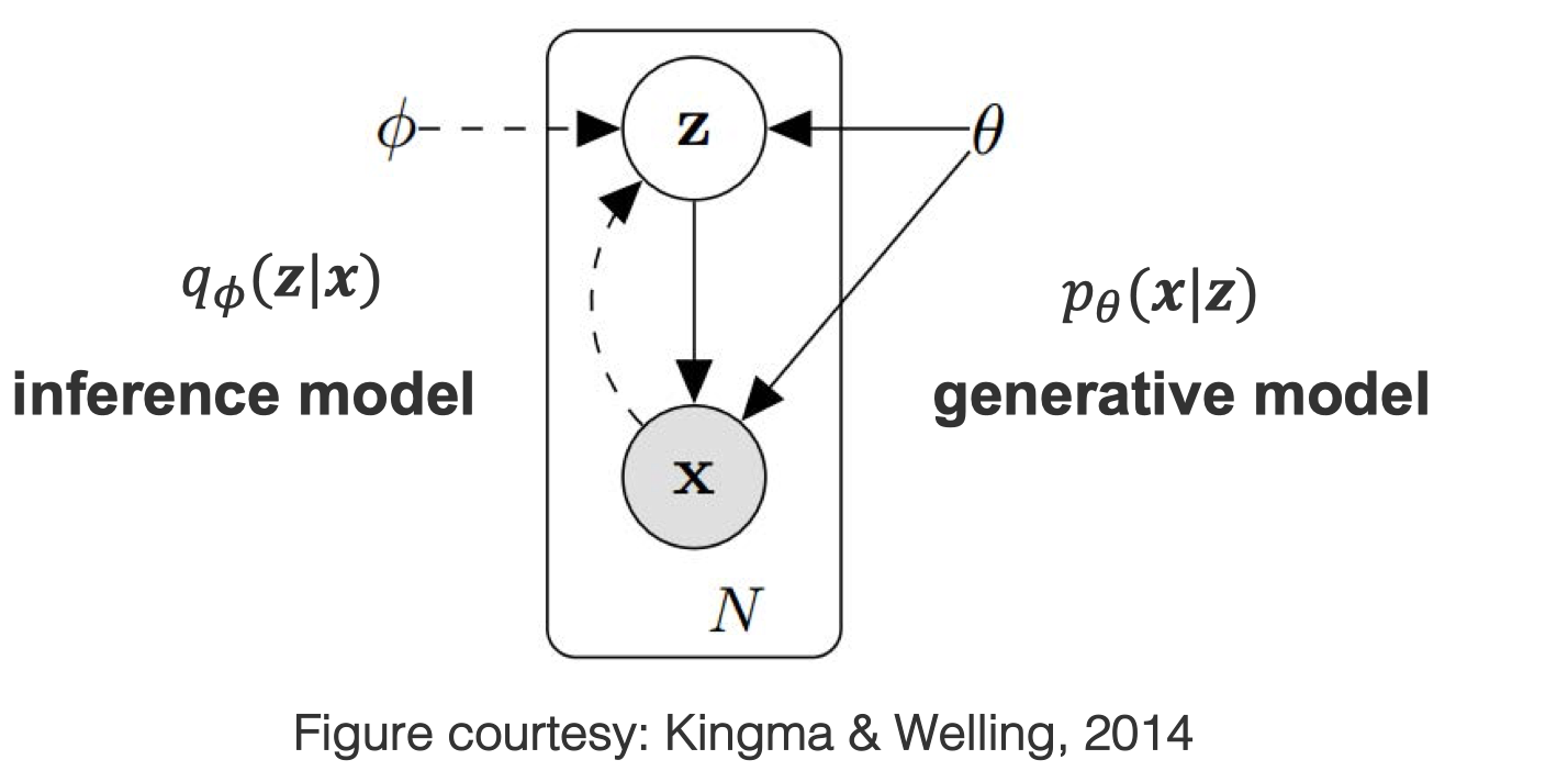
The idea here is simple. Autoencoder is not generative but we can make it generative by using variational inference. We can use the inference model as encoder. Pass the generated data to letent space Z, and decode the data using generative model.

Now, we want to estimate the true parameter of θ of the generative model. The question is how to represent it?

1. We can chose a simple prior p(z) like normal distribution.

2. Then we can train the model by maximizing the likelehood of training data: $p_{\theta}(x) = \int_{}^{}p_{\theta}(z)p_{\theta}(x

   z)dz$

Reparameterization Trick

To enable backpropagation through stochastic sampling, VAEs use the reparameterization trick:

\[z = \mu(x) + \sigma(x) \cdot \epsilon, \quad \epsilon \sim \mathcal{N}(0, I)\]

This reformulation allows gradients to flow through ( \mu(x) ) and ( \sigma(x) ), making the sampling operation differentiable and trainable with gradient descent.

Generating from a VAE

After training, you can generate new data as follows:

1. Sample a latent vector ( z \sim p(z) ), often a standard Gaussian.

2. Pass ( z ) through the decoder to get ( x’ \sim p(x

   z) ).

This enables the model to create novel data that resembles the training distribution.

GAN Architecture and Objective

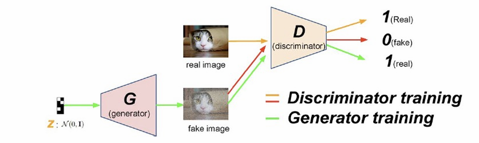
GANs consist of:

• A Generator ( G(z) ): maps random noise ( z \sim p(z) ) to data space, producing fake samples.
• A Discriminator ( D(x) ): attempts to distinguish real data from fake data.

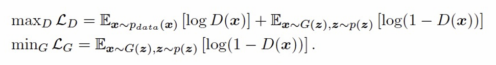
The generator learns to fool the discriminator; the discriminator learns to detect the fakes. Training is formulated as a minimax game:

\[\min_G \max_D \; \mathbb{E}_{x \sim p_{\text{data}}}[\log D(x)] + \mathbb{E}_{z \sim p(z)}[\log(1 - D(G(z)))]\]

This adversarial setup allows GANs to learn a rich, implicit distribution over data without explicitly modeling ( p(x

z) ).

Generative Adversarial Networks (GANs)

Key Points:

• Generative Adversarial Networks (GANs) provide a framework where two models (Generator and Discriminator) are trained simultaneously in a minimax game.
• The Generator attempts to produce samples that mimic the true data, while the Discriminator attempts to distinguish between real and fake samples.
• This process eventually yields a Generator that can produce highly realistic samples.
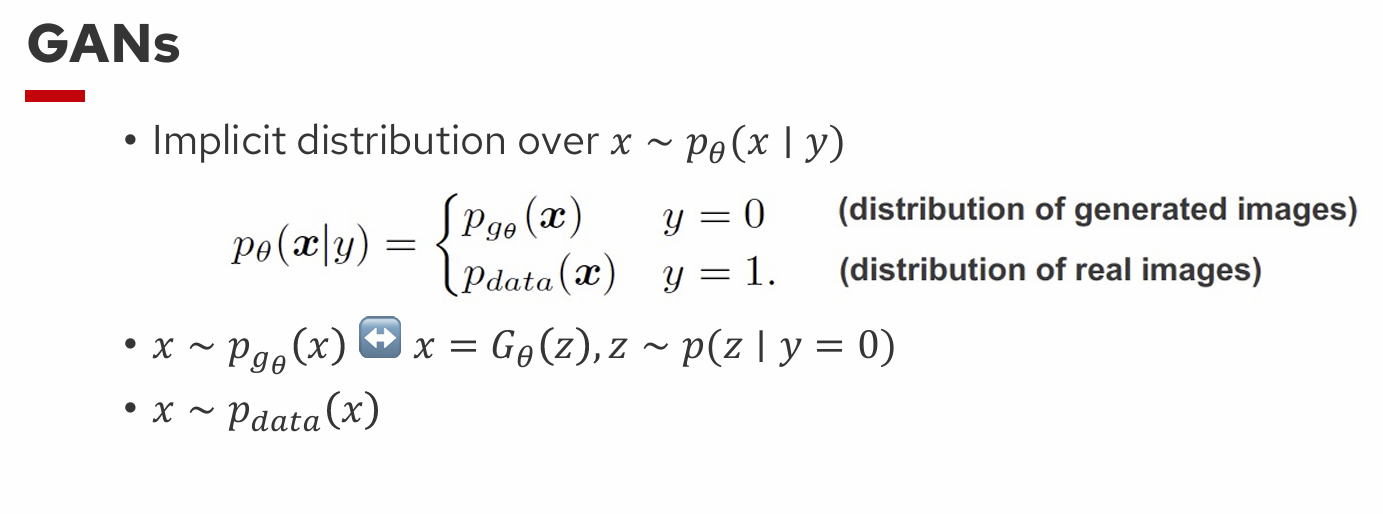
• The data distribution is “implicit”: meaning $p(x)$ isn’t parameterized directly.
• Sampling a latent variable $\mathbf{z}$ from a prior $\mathcal{N}(0,I)$ and mapping it through a generator $G(\mathbf{z})$ is done to obtain synthetic samples $\mathbf{x}$.
• Notation:
  • $\mathbf{x} \sim p_{\text{data}}(\mathbf{x})$
  • $\mathbf{x} = G(\mathbf{z}); \quad \mathbf{z} \sim p(\mathbf{z})$
• The Generator $G$ tries to transform noise $\mathbf{z}$ into data-like samples.
• The Discriminator $D$ evaluates whether a sample is real or generated.
• Training objective:

Slide 43: Training objective.

Slide 43: Outline of the generator-discriminator framework.

• The discriminator’s loss provides a training signal for the generator and therefore no explicit likelihood function is needed.
• Potential challenges:
  • Training instability due to the minimax setup.
  • Mode collapse where the generator produces a narrow set of outputs.
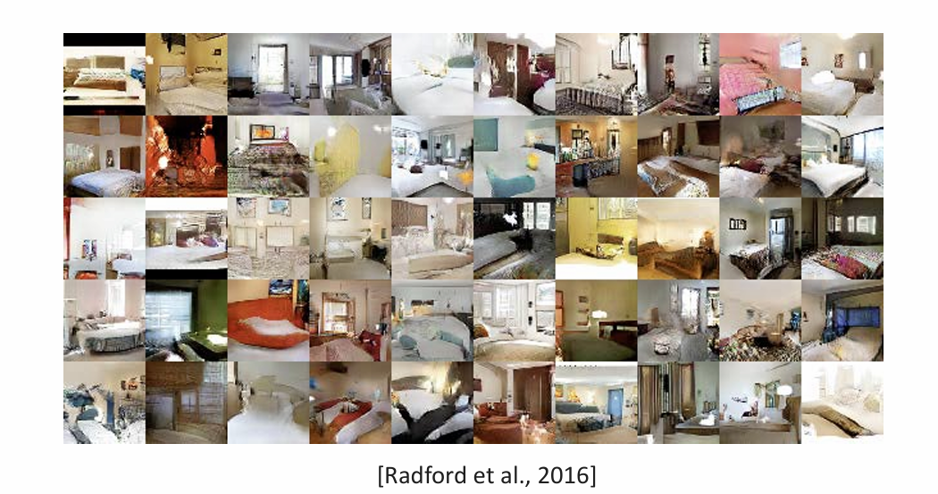
• DCGANs (Deep Convolutional GANs) produce realistic-looking images, illustrating how powerful adversarial training can be for generating image data.

Slide 45: Example Results.

GANs and VAEs: A Unified View

Key Points:

• Both are deep generative models but differ in how they learn:
  • VAEs: learn an explicit density by maximizing ELBO.
  • GANs: learn an implicit density via adversarial training.
• There have been attempts to combine these approaches (e.g., VAE-GAN hybrids).

Slide 47: GANs Revisited.

• Generator parameters define a mapping from latent space $\mathbf{z}$ to data space $\mathbf{x}$.
• The model distribution is implicitly defined by the transformation $G$ and the prior on $\mathbf{z}$.

Variational EM vs GANs

Key Points:

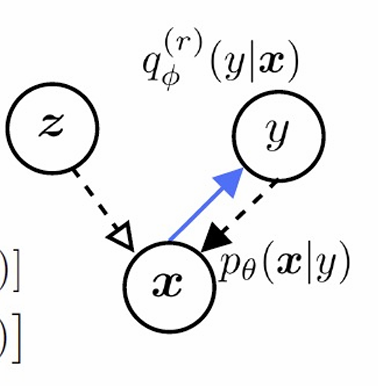
• The Discriminator can be viewed as a variational distribution $q_\phi(y \mid \mathbf{x})$, distinguishing real vs. generated.
• The Generator is used to a model that samples $\mathbf{x}$ by $\mathbf{x} = G(\mathbf{z}), \mathbf{z}\sim p(\mathbf{z})$.
• This interpretation draws parallels to EM, but the discriminator and generator have separate objectives.

Slide 48: GANs rewritten.

Slide 50: GANs vs VAEs.

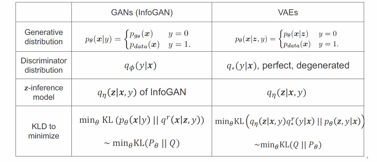
• Variational EM:
  • Single objective for both model ($\theta$) and variational distribution ($\phi$).
  • Extra prior regularization from $p(\mathbf{z})$.

  • Has a “reconstruction” term: it explicitly maximizes $\log p(x \mid z)$ with $z \sim q(z

    x)$.

• GAN:
  • Two objectives: the generator wants to fool the discriminator, and the discriminator wants to detect fakes.
  • No explicit prior penalty on $z$ for the reconstruction itself—rather, $z$ is drawn from $p(\mathbf{z})$.
  • Minimizes an adversarial loss instead of a direct $\log p(x\mid z)$ objective.

Slide 51: Mode Covering vs Mode dropping (mode collapse).

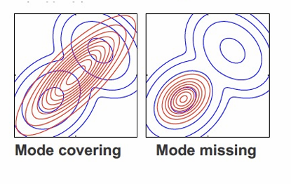
• VAEs can produce more “blurry” but comprehensive coverage (mode covering).
• GANs produce sharper images but risk missing entire modes (mode dropping).

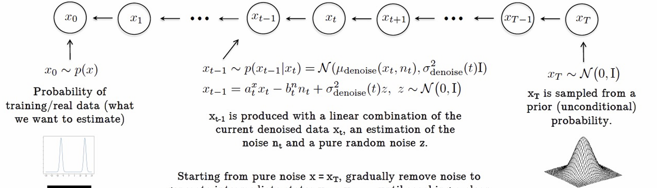
Diffusion Models

Key Idea:

• The forward process adds noise to data step-by-step, destroying structure.
• The backward process progressively denoises, reconstructing data from pure noise.

• These models are known for producing extremely high-fidelity generated samples (images, etc.).

• Training:
  • Often framed as predicting the added noise at each step, similar to a score-matching approach.
  • Once trained, sampling involves reversing the noise steps to create data-like samples from random noise.

Slide 53: Diffusion Model: Backward Process.

Slide 54: Diffusion Model: Forward Process.